Cracking the Code: Testing Averages When Your Data Isn’t All There

Hey there! Ever looked at a dataset and noticed some bits are just… missing? It happens more often than you’d think in the real world. Maybe someone didn’t answer a question, a sensor failed, or a measurement wasn’t taken. Dealing with this missing data is a huge part of what we statisticians grapple with. It’s like trying to solve a puzzle when you don’t have all the pieces.

Now, imagine you’re not just interested in the overall average of everything, but maybe the average of a specific *subset* of your variables – what we call a “sub-mean vector.” And to make things extra tricky, the data isn’t missing randomly everywhere; it follows a particular pattern. The kind we’re talking about here is called “two-step monotone missing data.” Sounds complex, right? Well, it can be, but let’s break it down.

This kind of missing data pattern often shows up in longitudinal studies or surveys where participants drop out or skip later sections. You might have a group with complete data on everything, and another group that only completed the first few sets of measurements. It’s structured, but incomplete.

When you have this specific missing pattern and you want to test hypotheses about the average of just *some* of your variables (the sub-mean vector), the standard statistical tests designed for complete data suddenly don’t quite fit. It’s like having the right key, but the lock has changed shape slightly.

Our goal in this work was to figure out how to extend those classic, reliable tools to handle this exact scenario. We wanted to build new test statistics that could confidently tell us if a subset of our averages was significantly different from a hypothesized value, even with this two-step missing data pattern.

The Missing Piece of the Puzzle: Understanding the Data

So, what does this “two-step monotone missing” thing actually look like? Picture your data as a big spreadsheet. In our case, we have two groups of rows (observations).

• The first group (let’s call it (N_1)) has data for *all* your variables. Everything is there, neat and tidy.
• The second group (let’s call it (N_2)) only has data for a *subset* of the variables – the first few columns, if you like. The rest are blank (*missing*).

The “two-step” refers to the two groups ((N_1) and (N_2)), and “monotone” means that if a variable is missing for a person in the second group, all subsequent variables are also missing. It’s a specific, ordered pattern of incompleteness. We assume this missingness happens “completely at random,” meaning the reason data is missing doesn’t depend on the values themselves.

Why Standard Tests Fall Short

Classic statistical tests, like the famous Rao’s U-statistic (which is related to Hotelling’s T²), are designed assuming you have a full matrix of data. When you introduce missing values, especially in a structured way like this, the calculations for things like sample means and covariance matrices get complicated. You can’t just plug the incomplete data into the old formulas and expect reliable results.

Researchers before us had looked at this problem, proposing tests like the likelihood ratio test. That’s a solid approach, but we wondered if we could build a test based directly on the *structure* of Rao’s U-statistic, adapting it specifically for our two-step missing pattern. Think of it as creating a new, specialized key based on the design of the original, but shaped for the new lock.

Building New Tools: Our Approach

We decided to construct new test statistics. Our approach was to take the core idea behind Rao’s U-statistic and incorporate components that could handle the missing data. We did this by using something called a “Hotelling’s T²-type statistic,” which is a version of the classic T² adapted for missing data scenarios.

We focused on testing different hypotheses about the sub-mean vector. For instance, testing if the average of variables 2, 3, and 4 (given variable 1’s average is known) is a certain value. Or testing the average of variables 3 and 4, or just variable 4, under similar conditions. We built specific statistics, which we called (U_1) and (U_{(123)}), to tackle these different test scenarios.

Peeking into the Future: Stochastic Expansions

Now, the tricky part: figuring out the *distribution* of these new test statistics. When you have complete data, classic statistics often follow well-known distributions like the F-distribution or Chi-squared distribution, especially with large sample sizes. These distributions give us the critical values needed to decide if our test result is statistically significant.

For our new statistics with missing data, their exact distributions are complicated. However, for *large* sample sizes, we can approximate their behavior. We used a powerful mathematical technique called “stochastic expansion.” This is essentially a way to approximate a complex random variable (our test statistic) using a series of simpler terms. It helps us understand how the statistic behaves as the sample size grows.

By deriving these expansions, we could show that, for large samples, our new test statistics behave approximately like a Chi-squared distribution. This is fantastic because the Chi-squared distribution is well-understood, and we have tables (or software) to find the critical values.

Making it Better: Approximations and Corrections

Based on the stochastic expansions, we could propose “approximate upper percentiles.” These are the estimated critical values – the thresholds our test statistic needs to cross to declare a result statistically significant at a certain confidence level (like 95% or 99%). We denote these approximate percentiles as (u^*_{1}(alpha)) and (u^*_{(123)}(alpha)), where (alpha) is the significance level.

But what about smaller sample sizes? The large-sample approximation might not be accurate enough. To improve things, especially for more modest datasets, we also looked into applying a “Bartlett correction.” This is a standard technique in statistics that adjusts a test statistic to make its distribution closer to the target (in our case, the Chi-squared) for finite sample sizes. We derived the formulas for these corrected statistics, (widetilde{U}_{1}) and (widetilde{U}_{(123)}). The hope was that these corrected versions would give more accurate results when we don’t have massive amounts of data.

Putting it to the Test: Simulations Galore!

Theory is great, but you need to see how things work in practice! So, we ran extensive Monte Carlo simulations. This involves generating lots and lots of artificial datasets that mimic the two-step monotone missing pattern, where we *know* the true underlying averages. Then we apply our new test statistics and see how often they lead us to the right conclusion (or, importantly, how often they lead us to the wrong conclusion when the null hypothesis is true – this is the “Type I error”).

We tested various scenarios: different numbers of variables in each part ((p_1, p_2, p_3, p_4)), different total sample sizes ((N_1, N_2)), and different ratios of complete to incomplete data.

Here’s what we generally saw:

• Our proposed approximate percentiles ((u^*)) worked quite well, especially when the sample sizes ((N_1) and (N_2)) were large. The larger the sample, the better the approximation, which makes sense given they were based on large-sample theory.
• The accuracy could depend on the dimensionality. Sometimes, having more variables made the approximation a bit less accurate, but it still held up reasonably well.
• The Bartlett correction ((widetilde{U})) often provided a better approximation to the target Chi-squared distribution, particularly for smaller sample sizes or certain configurations of variables. It helped “correct” the statistics to behave more like we expect.
• We also looked at the “power” of the tests – how well they detect a *real* difference in the sub-mean vector when one exists. Our simulations showed that both the original proposed statistics and the Bartlett-corrected versions had similar power, which is good news. The correction primarily helps with getting the significance level right, not necessarily the power to detect a difference.

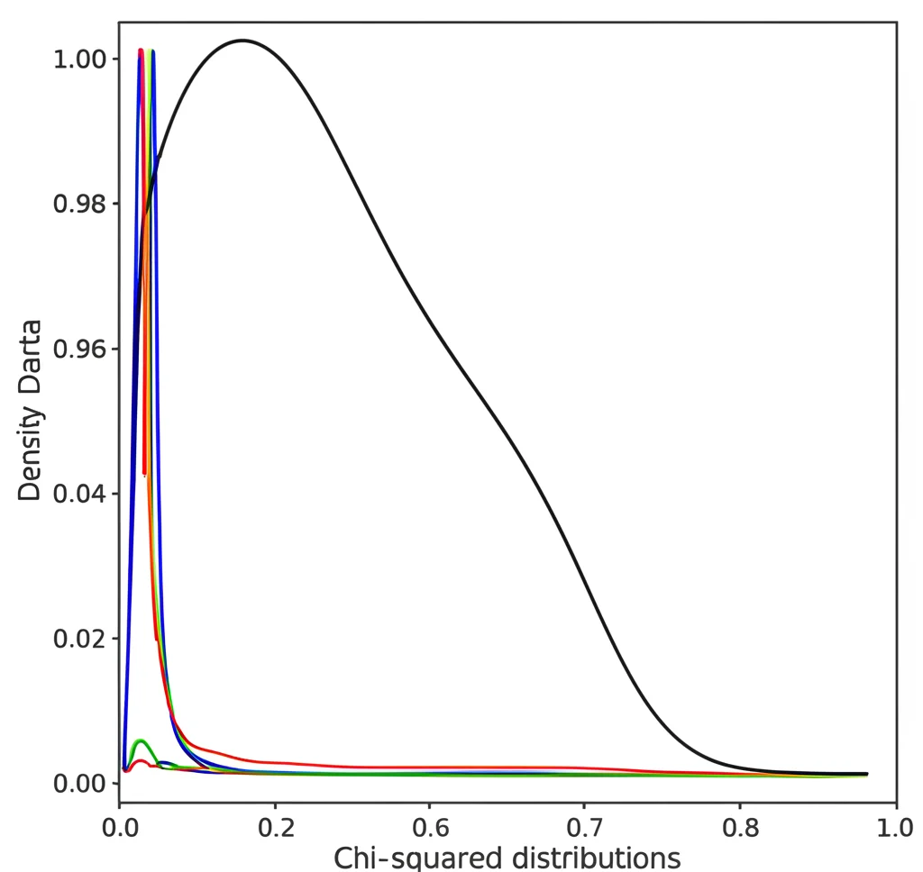
We even compared the *shape* of the distribution of our statistics from the simulations to the theoretical Chi-squared distribution using density plots (basically, graphs showing how frequently different values of the statistic occurred). As expected, with large sample sizes, the histograms of our statistics lined up nicely with the smooth curve of the Chi-squared distribution. For smaller samples, the Bartlett-corrected versions often provided a better match.

Real-World Taste Test: The Wine Example

To show how you might actually *use* these new tools, we applied them to a real dataset: measurements of Portuguese red wine (Vinho Verde). The original data had 1599 observations, but we created a smaller example dataset with our specific two-step monotone missing pattern, using 20 observations total (10 complete, 10 incomplete). We focused on variables like fixed acidity, volatile acidity, density, and pH.

We set up a hypothesis about the average values of some of these wine properties, assuming the average fixed acidity was known (since it comes from the grapes). We then computed our new test statistic, (U_1), and the Bartlett-corrected version, (widetilde{U}_1), for this wine data.

We compared our calculated statistic values to the approximate critical values ((u^*_1)) and the critical values from the standard Chi-squared distribution (which the Bartlett-corrected statistic aims for).

The results showed how using the different critical values could influence the conclusion. Depending on whether we used the standard Chi-squared critical value or our newly derived approximate percentiles, and whether we used the original statistic or the corrected one, the decision to reject or not reject the hypothesis could change, especially near the significance boundary (like 0.05). This highlights the importance of using the appropriate critical values derived for the specific missing data structure.

Wrapping It Up: What We Found

So, what’s the takeaway? We successfully developed new test statistics based on the structure of Rao’s U-statistic, specifically designed for testing sub-mean vectors when you have two-step monotone missing data.

We figured out how these statistics behave for large samples using fancy math (stochastic expansions) and used that to provide handy approximate critical values. We also proposed a Bartlett correction to make things more accurate for smaller datasets.

Our simulations confirmed that these new tools work well. The approximate critical values are good, especially for large samples, and the Bartlett correction helps improve accuracy. The power of the tests is solid.

Ultimately, this work provides researchers and analysts with reliable methods to test hypotheses about parts of their average vectors in a common missing data scenario where standard tests fall short. It’s another step in making sure we can still get meaningful insights even when our data isn’t perfectly complete.

Source: Springer