Unlocking Complex Systems: Mittag-Leffler, Diffusion, and Our Math Adventure

Hey there! Ever wonder how scientists and mathematicians tackle really complex stuff? You know, things that don’t just follow simple, straight lines but have a bit of a memory or depend on their whole past history? That’s where something called fractional calculus comes into play. Think of it as calculus, but with a twist – instead of just whole number derivatives (like the first or second derivative), you can have derivatives of any order, like 0.5 or 0.9!

We recently embarked on a little adventure exploring how a particular type of fractional derivative, one tied to a cool function called the Mittag-Leffler function, can help us understand things like how chemicals react or how stuff spreads out over time and space. We’re talking about linear kinetic models and diffusion equations here. It’s pretty neat how these advanced mathematical tools can give us a clearer picture of the world around us.

A Little Bit About Fractional Calculus

So, why bother with fractional calculus? Well, the classical, integer-order calculus we all learned is great for describing systems where the future only depends on the present state. But lots of real-world systems remember their past! Materials that get fatigued, how electromagnetic fields behave, even how substances move through biological tissues – they all have this ‘memory’ aspect. Fractional derivatives are the perfect tools to capture this.

Over the years, folks have come up with different kinds of fractional derivatives. There’s the classic Caputo and Riemann-Liouville, which are super useful for things like damage and fatigue. But sometimes, for materials that are really mixed up or have structures on different scales, these traditional ones don’t quite cut it. Then came the Caputo-Fabrizio derivative, which has a nice, non-singular kernel, but it’s still kind of ‘local’ because its kernel only depends on the difference in time.

In 2016, Atangana and Baleanu shook things up by proposing a new approach using the generalized Mittag-Leffler function. Their goal? To create fractional operators with kernels that are both non-singular (meaning they don’t blow up at certain points) and non-local (meaning they truly capture that memory effect). These Atangana-Baleanu-Caputo fractional derivatives (ABCFD) have been quite the hit because they do a fantastic job describing systems with this Mittag-Leffler memory.

Now, like anything new, the ABCFD has its critics. Some argue it doesn’t play nice with some fundamental rules of fractional calculus, like having a corresponding convolution integral. Also, the derivative’s value at the very start (time t=0) is always zero, which might feel a bit restrictive for certain models. But despite these points, the ABCFD has proven itself effective in modeling complex systems, showing up in studies on hybrid fractional differential equations, non-linear models, and even the dynamics of alcohol consumption (yes, math gets everywhere!).

Putting it to Work: Kinetic Models

So, what did we do with this fancy ABCFD? We decided to test it out on some linear fractional kinetic models. These models are super common for describing rates – like how fast a chemical reaction happens, how quickly a radioactive substance decays, or even how populations grow or shrink. We applied the ABCFD to three basic kinetic models.

Using tools like the Laplace transform, we found the solutions for these models. Here’s the cool part: we showed that if you set the fractional order (that ‘twist’ number) back to 1, you get the exact same solutions you’d get with classical, integer-order calculus! This confirms that fractional derivatives are indeed a generalization of the traditional ones.

• The first model showed a system in equilibrium – basically, nothing changes over time, which makes sense for a stationary model.
• The second model showed something increasing linearly with time, just like you’d expect in a classical linear growth scenario when the fractional order is 1.
• The third model represented something decreasing over time (like decay or cooling), but with the added ‘memory’ effect from the Mittag-Leffler kernel. When the fractional order is 1, it reduces to the familiar exponential decay.

We also compared these results with what you get using the classical Caputo fractional derivative (CFD). While both methods recover the classical solution at order 1, their behavior differs for fractional orders between 0 and 1, highlighting the unique properties of the ABCFD’s kernel.

Diffusion, Diffusion Everywhere

Next up: Diffusion equations. These are essential for modeling how quantities like heat, particles, or chemicals spread out over space and time. They’re used in everything from understanding star formation and plasma behavior in space to how medications move through your body. Solving these equations, especially when they involve fractional derivatives or are in multiple dimensions (like 2D or 3D), can be quite tricky.

Since finding exact solutions is often impossible, researchers rely on clever methods to find really good approximate solutions. We’re talking about techniques like the Adomian decomposition method (ADM), the iterative method (IM), and the homotopy perturbation method (HPM). These methods are known for giving you solutions in the form of a series that converges quickly to the true solution.

Sometimes, you can make these methods even more powerful by combining them with transforms like the Laplace transform or the Sumudu transform. For example, coupling the iterative method with the Laplace transform gives you the iterative Laplace transform method (ILTM).

Our Secret Weapon: The HPSTM

For our diffusion problem, we used a modified technique: the Homotopy Perturbation Sumudu Transform Method (HPSTM). This method is a powerful combo of the Homotopy Perturbation Method (HPM) and the Sumudu transform, specifically using the Sumudu transform tailored for the ABCFD (which, remember, has that cool Mittag-Leffler kernel!).

Why is this combination great? You get the rapid convergence benefits of HPM along with the power of the Sumudu transform, and when applied to the ABCFD, it brings in those valuable memory effects that are crucial for modeling complex systems like viscoelastic materials or anomalous diffusion processes.

The basic idea is pretty clever. You apply the Sumudu transform to your fractional differential equation, use the initial condition, and then apply the homotopy perturbation method. This involves expanding the solution into a power series using a parameter, and then comparing terms to find approximations. The result is a solution in the form of a series where each term is relatively easy to compute.

Solving the Diffusion Puzzle

We applied this HPSTM to solve two-dimensional and three-dimensional fractional diffusion equations using the ABCFD. We started with the equations and their initial conditions, applied the Sumudu transform of the ABCFD, and then used the HPM expansion.

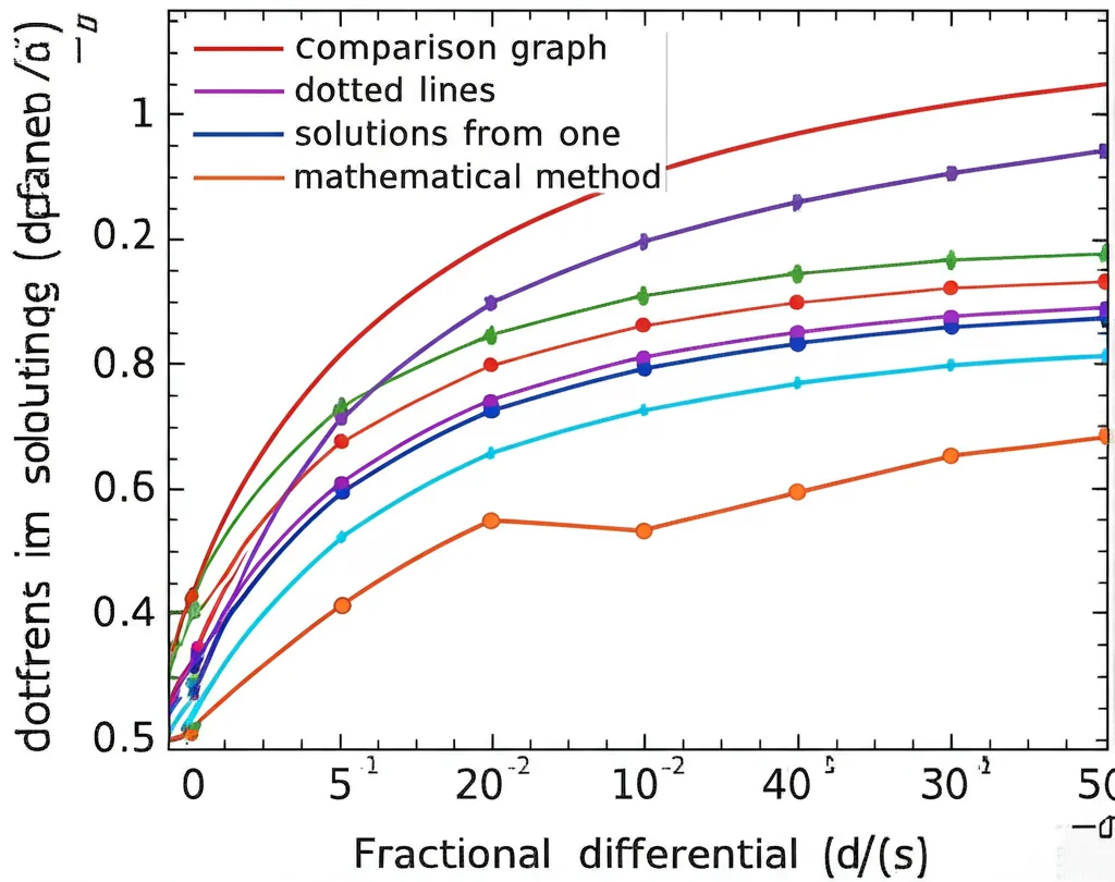
We used Mathematica software to visualize our results, plotting both 2D and 3D graphs. What we saw was pretty encouraging! The approximate solutions we got from the series were very close to the exact solutions, especially as we included more terms in the series. This means the method is effective and the series converges nicely.

Just like with the kinetic models, we made sure to check what happens when the fractional order is set to 1. And guess what? We recovered the classical, integer-order diffusion equation solutions! This further validates that the fractional approach is a true generalization.

We also played around with different values for the fractional order (like 0.85, 0.90, 0.95) to see how the solutions behave. As the fractional order gets closer to 1, the approximate solutions naturally get closer to the classical exact solution.

ABCFD vs. CFD: The Showdown

One of our main goals was to see how the ABCFD stacks up against the classical Caputo fractional derivative (CFD) for these specific diffusion problems. We compared the approximate solutions obtained using both methods.

What did we find? For the diffusion equations we studied, the classical Caputo method seemed to converge to the exact solution a bit faster than the ABCFD method. This might suggest that for problems where rapid convergence is key, the classical Caputo method could be more suitable, especially in the initial stages.

However, this doesn’t mean the ABCFD is less useful! Its unique ability to capture non-local behaviors and those specific memory and hereditary properties makes it invaluable for other types of problems where these features are dominant. The choice between the two really depends on the specific system you’re trying to model and which properties are most important to capture accurately.

We also calculated the absolute errors between the exact and approximate solutions, confirming that increasing the number of terms in the series significantly reduces the error, making the approximate solutions very accurate.

Looking Ahead: Future Possibilities

So, where does this leave us? We successfully used the HPSTM with the ABCFD to solve kinetic models and diffusion equations, showing the method is effective and the solutions converge. We also highlighted the differences and similarities between the ABCFD and the classical CFD.

Our findings pave the way for exciting future work. We can use this as a jumping-off point to create even more precise and efficient numerical techniques. Maybe combine HPSTM or other methods like the Adomian decomposition method with different transforms, like the Elzaki transform, to tackle even more complex linear and non-linear fractional differential equations.

The applications of fractional diffusion equations are growing rapidly in fields like biology, engineering, and physics, especially for processes that don’t fit the standard diffusion model. We’re keen to explore new applications, perhaps venturing into areas like financial mathematics, control theory, or materials science. And of course, there’s always room to improve the computational efficiency and accuracy of these methods to make them even more practical for real-world use.

Conclusion

Diving into the world of fractional calculus, particularly with the Mittag-Leffler-based ABCFD, has been a fascinating journey. We’ve seen how it provides a powerful framework for modeling systems with memory, and how methods like the HPSTM can effectively solve the resulting equations. While the classical Caputo method might win in a speed race for some specific problems, the ABCFD’s unique properties make it indispensable for others. It’s clear that fractional calculus is a vital tool for understanding the complex, interconnected dynamics of our universe, and we’re excited to see where these mathematical adventures take us next!

Source: Springer