Unlocking Sound Secrets: A Hybrid Approach to Alpha Cabin Absorption
Hey there! Let’s talk about sound, specifically how things soak it up. If you’ve ever been in a really quiet car, you know how much effort goes into making that happen. A huge part of it involves using special materials that absorb sound. But how do you figure out *how good* a material is at this job, especially when it’s going into something as complex as a car interior?
In the automotive world, we often use these neat little rooms called “alpha cabins” to test sound-absorbing materials. Think of them as mini reverberant chambers. They’re super handy because they’re smaller and fit the kind of oddly shaped samples you find in cars. The catch? They’re not like the big, standard rooms used in building acoustics, which create a perfectly spread-out, or ‘diffuse’, sound field. Alpha cabins are smaller, and that can mess with the sound field, especially at lower frequencies.
Since there aren’t standard rules for measuring absorption in these non-diffuse conditions, we needed a clever way to get accurate numbers. That’s where this cool new approach comes in – a hybrid method that mixes two different ways of looking at sound waves: the time-harmonic (like looking at a single, steady note) and the time-domain (like watching the sound fade away over time).
The Automotive Sound Challenge
Making cars quiet isn’t just about luxury; it’s also about protecting the vehicle’s structure from constant vibrations and noise. The classic way to measure a material’s absorption is using something called a Kundt tube. It’s great, but it only tells you how a flat sample absorbs sound coming straight at it (normal incidence). Car parts aren’t usually flat, and noise hits them from all sorts of angles. So, the Kundt tube data doesn’t give the full picture.
For a better idea of how a material performs in a real-world setting, you’d ideally use a large reverberation room to measure its performance in a diffuse field. Alpha cabins are the automotive industry’s answer – smaller, more affordable, and better suited for testing car-specific samples. But their size introduces issues like sound bending around the edges of the sample (diffraction) and that tricky non-diffuse sound field I mentioned earlier. This is particularly problematic at low frequencies, where car noise can be a real headache.
This is where numerical simulation becomes our best friend. It lets us peek inside the alpha cabin and see exactly what the sound is doing, even with small, oddly shaped samples and at those challenging low frequencies. Instead of older methods like ray tracing (imagine bouncing light rays) or image sources, we’ve developed something different.
Our Two-Stage Hybrid Solution
We decided to try a hybrid numerical approach. It’s like tackling the problem in two steps using a method called Finite Element Method (FEM). FEM is fantastic for breaking down complex shapes and physics into smaller, manageable bits.
Step One: Setting the Scene (Time-Harmonic)
First, we simulate the sound field inside the alpha cabin while the sound source (like a speaker) is on. We use a ‘time-harmonic’ approach here. Think of it as calculating the steady state of the sound waves at a specific frequency. What’s a bit different is that we focus on the *displacement* of the air particles, not just the pressure. This ‘displacement-based’ formulation turns out to be really helpful, especially when dealing with materials that absorb sound (they have an ‘impedance’ boundary condition).
We use special FEM elements called Raviart-Thomas elements for this. They have some nice mathematical properties that make the simulation more stable and efficient, avoiding certain numerical glitches you sometimes see.

Step Two: Watching the Sound Fade (Time-Domain)
Once we know the steady sound field from Step One, we turn the source off (in our simulation, of course!). Now, we switch to a ‘time-domain’ simulation. This means we watch how the sound energy decays over time. The cool part is that we use the results from Step One (the displacement and velocity fields) as the starting point for this decay simulation. This links the two stages together beautifully.
We use the same type of FEM elements and a reliable time-stepping method (like the Newmark scheme) to accurately track the sound’s decay without introducing numerical errors that could make it look like the sound is fading when it’s not.
What I find particularly neat about this hybrid approach is that it combines the strengths of both methods. The time-harmonic part lets us analyze the sound field’s character (is it diffuse or not?) at different frequencies, which is crucial for understanding the alpha cabin’s limitations. The time-domain part, initialized smartly, allows us to calculate the decay efficiently without simulating an unnecessarily long time.
Measuring the Quiet: From Decay to Absorption
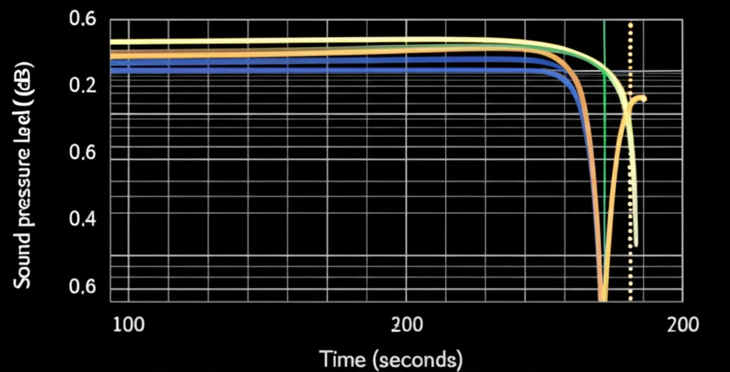
The key to finding the absorption coefficient in a room is the reverberation time. That’s the time it takes for the sound pressure level (SPL) to drop by 60 decibels after the source stops. Our simulation gives us the pressure field over time, so we can calculate the SPL decay.
There are different ways to measure this decay, based on standards like ISO 354 and ASTM C423. The ISO standard strictly requires measuring the time to drop 60 dB, which can mean simulating for a *very* long time if the material doesn’t absorb much. The ASTM standard is more practical; it looks at the decay rate over shorter time windows using local averages of the SPL. We also looked at other methods like global regressions.
What we found is that the ASTM approach, using those local averages, is much more robust. Measuring SPL at single points in time can be sensitive to tiny numerical wiggles, leading to inaccurate reverberation times. The local averaging smooths things out and gives a much more reliable decay rate.
Turning Time into a Number: Sabine vs. Millington
Once we have the reverberation time (`t_rev`) from the decay simulation, we use classic formulas to estimate the absorption coefficient (`alpha`) of the material sample. The two main ones are the Sabine formula and the Millington formula.
- Sabine Formula: This is a simpler formula, often used, but it can sometimes overestimate absorption, especially for materials that absorb a lot.
- Millington Formula: This one is generally considered more accurate, particularly when absorption values are low.
These formulas also need information about the room size (volume and surface area) and whether the sound field is diffuse or not. In our case, since the alpha cabin isn’t perfectly diffuse, we have to consider how that affects the calculation. When the cabin is empty (no absorbing sample), our simulation shows no energy decay (because the walls are modeled as rigid), so the empty reverberation time is essentially infinite, simplifying the formulas a bit.
Putting Our Hybrid Method to the Test
We ran several tests to see how well our hybrid method works. We started with a simple 2D simulation where we knew the exact answer – a ‘manufactured’ case. This helped us validate that the method and our implementation were correct. We saw that using the ASTM standard’s local averages combined with the Millington formula gave the most accurate results compared to our known solution.
Next, we tested it on a 2D case using data from a real fibrous material (like the stuff used in cars). We modeled its sound-absorbing properties using a simplified impedance model that fits experimental data from a Kundt tube. Again, the hybrid method, particularly with ASTM local averages and Millington, did a great job of predicting the absorption coefficient, showing good agreement with the experimental Kundt tube data (which, remember, is for normal incidence).
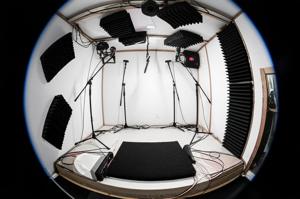
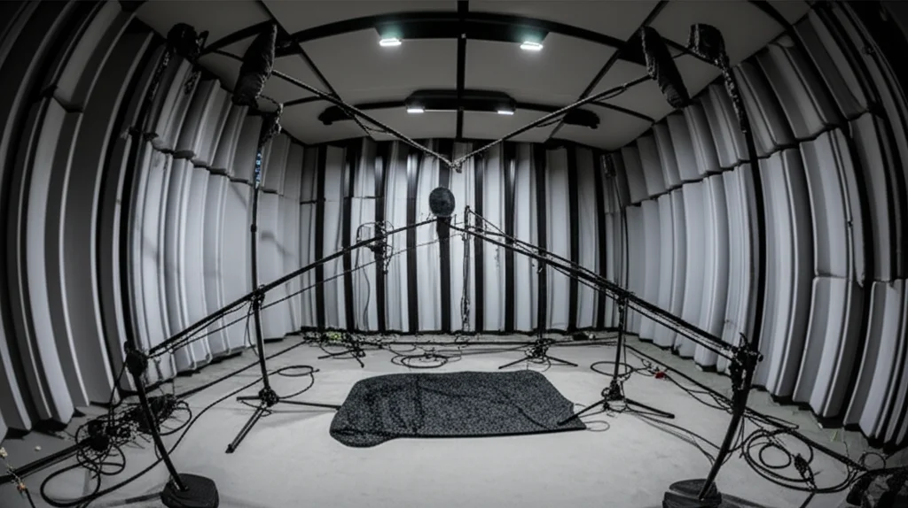
Finally, we stepped up to a realistic 3D alpha cabin geometry, complete with diffusers and multiple speaker/microphone locations. We used the same fibrous material data. Even though this alpha cabin is smaller than ideal for a perfectly diffuse field, our hybrid method could still compute the reverberation times. When we calculated the absorption coefficient using the diffuse field assumption (as you would typically try to do in an alpha cabin), the results showed a trend qualitatively similar to the experimental Kundt tube data. And just like in the 2D tests, Millington’s formula gave results closer to the experimental trend than Sabine’s.
These tests confirmed that our hybrid time-harmonic/time-domain approach is a solid numerical tool. It can help engineers characterize how sound-absorbing materials will perform in alpha cabins, whether the sound field is perfectly diffuse or not. And the winning combination for getting the most reliable numbers? Using the ASTM standard’s local Leq averages to calculate the decay rate and then plugging that into Millington’s formula.
Wrapping It Up
So, there you have it. Measuring sound absorption accurately in the specific environment of an automotive alpha cabin is challenging. Traditional methods have limitations, and the cabins themselves aren’t standard. Our hybrid time-harmonic/time-domain simulation approach, built on displacement-based FEM and validated against experimental data, offers a powerful way to tackle this. By carefully simulating how sound builds up and then decays, and using robust methods like ASTM’s local averaging and Millington’s formula to interpret the results, we can get reliable estimates of a material’s absorption coefficient. This is a big step forward for automotive acoustics, helping engineers design quieter, more comfortable cars.

Source: Springer